Physical Modeling Synthesis

What is physical modeling synthesis?

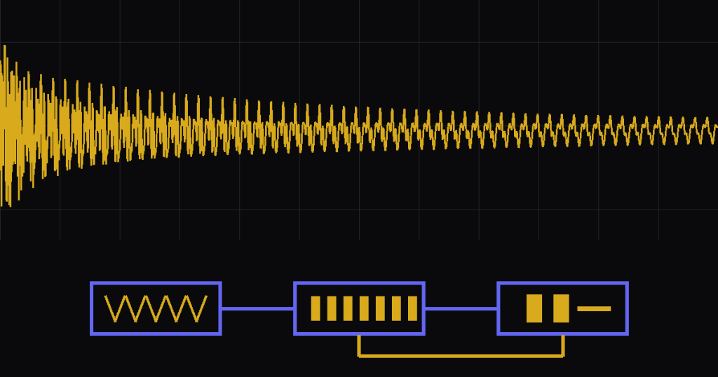
Physical modeling synthesis is a way of making sound by simulating the object that vibrates, instead of playing back a recording or filtering a raw waveform. An exciter, such as a pluck, a strike, a bow or a breath, drives a resonator, such as a string, a tube, a bar or a drum head. The synth computes the result as you play.

Stanford’s CCRMA puts the difference in one line: “With physical modeling it is the actual physics of the instrument and its playing technique which are modelled by the computer” (CCRMA, CLM tutorial: Physical Modelling Synthesis). A sample stores what an instrument sounded like once. Subtractive synthesis starts from a bright waveform and filters it. A physical model stores neither: it stores the instrument. British sources spell it physical modelling, and it’s the same thing.

The physical modeling instruments I’ve used myself are Applied Acoustics Systems’ Chromaphone and Strum. Below: how it works, the main techniques, four things I measured in a basic Karplus-Strong loop, and where to find physical modeling today.

How physical modeling works: exciter, resonator, coupling

Perfect Circuit’s explainer starts from the same split every model uses: “At the very basic, there are two components: an exciter, and a resonator” (Perfect Circuit, What is Physical Modeling?, September 2023). The exciter puts energy in. The resonator decides what that energy turns into.

That flips the roles you know from a classic synth. In a subtractive patch, the oscillator sets the pitch and the filter only colors it. Mutable Instruments’ Elements manual describes the opposite for modal synthesis: “In modal synthesis, the raw material is bursty and unpitched. What is truly responsible for the pitch of the note, and its timbre is the resonator” (Mutable Instruments, Elements manual). The burst can be as simple as a short click or a puff from a noise generator.

The best models add a third part: the coupling between the two. Sound On Sound’s 1997 explainer says full physical modelling “attempts to produce models for the driver, the resonator, and their interactions. This provides a feedback path which is not present in simpler models” (Sound On Sound, Physical Modelling Synthesis Explained, June 1997). A bow that sticks and slips on a string, or a reed that the air in the bore pushes back on, needs that feedback path.

Because you edit the object rather than the waveform, the controls are physical. Edinburgh’s NESS project puts it this way: “instruments are defined by geometrical and material parameters, few in number” (NESS project, University of Edinburgh).

The memory difference is real. Pianoteq shows it: Sound On Sound’s first review asked “Can an 8Mb plug-in really compete with the new generation of multi-Gigabyte sampled grand pianos?” (Sound On Sound, January 2007). Today Modartt lists the download at “~50 MB” (Modartt, Pianoteq).

The four main physical modeling techniques

Physical modeling is a family of methods, not one algorithm. They differ in how much of the physics they keep and how much computing they cost.

Karplus-Strong: a plucked string from a noise loop

The cheapest model of all. A short delay line full of random numbers is read out over and over, and each pass through a tiny averaging filter makes the noise ring like a string. It needs no multiplications, and Kevin Karplus says it ran two or three voices at once in real time on an 8080A microprocessor. The next section walks through it step by step.

Digital waveguides: strings and tubes as delay lines

A vibrating string or air column carries two waves moving in opposite directions, a solution to the wave equation that goes back to d’Alembert in 1747 (J. O. Smith, Physical Audio Signal Processing, CCRMA). In code, Smith writes, “The resulting computational model turns out to be a simple bidirectional delay line” (PASP, Digital Waveguide Models).

The trick that makes it cheap is to gather all the small losses along the string into one filter. In Smith’s example of a 100 Hz string, that “reduced computational complexity by three orders of magnitude, i.e., by a factor of 500 in this case” (PASP, Computational Savings). Waveguides are also the commercial success story. NESS calls them “the most successful application to date of physical modelling synthesis methods.” Stanford held the core waveguide patent, US 4,984,276 (Google Patents), and licensed it to Yamaha in 1989 (Stanford OTL newsletter, Autumn 1992).

Modal synthesis: a bank of ringing filters

Modal synthesis describes an object by its modes, the frequencies at which it likes to ring, and how fast each one dies. Smith defines the structure as “a parallel filter bank in which each filter section implements the transfer function of some resonant mode in the physical system” (PASP, Modal Representation).

If that sounds like a tuned band-pass filter bank, it is, and each mode is one partial in the additive sense. Modal models suit bars, plates, bells and drums, whose partials are not neatly harmonic. The Elements manual even names an analog ancestor. “A classic analog piece of equipment that used modal synthesis is the Roland TR-808 drum machine.”

Finite-difference and mass-spring models: the general case

The heaviest approach, and the oldest one for strings, solves the physics on a grid of points, step by step in time. Smith’s book dates “the earliest known digital models of vibrating strings” to “Pierre Ruiz and Lejaren Hiller ca. 1971” (PASP, Finite Difference Methods). Mass-spring networks, pioneered by Claude Cadoz’s CORDIS system in Grenoble, chain point masses together with springs instead.

These methods make few assumptions, so they can model almost anything. NESS: “Such methods, as they rely on virtually no simplifying hypotheses, are of great generality”, but they are far less efficient than digital waveguides. The cost can be extreme. According to Edinburgh’s supercomputing center, a 3D room model “requires 28 GB of memory and it takes 240 processor-cores of the order of 80 minutes of wall-clock time to produce one second of audio output” (EPCC, NESS project, April 2017). The same report notes that its brass models “can run faster than real-time”, so the cost depends on the model.

The Karplus-Strong algorithm, step by step

The Karplus-Strong algorithm makes a plucked-string sound from a delay line filled with noise. Each time the samples come round, neighboring samples are averaged, which smooths the noise into a decaying, pitched tone. It fits in a few lines of code.

1. Fill a delay line with N random numbers, with the average taken out, since the averager passes a DC offset at full level and it would never decay. Smith’s book defines Karplus-Strong proper as the case where the delay line’s starting contents “consist of random numbers” (white noise) (PASP, The Karplus-Strong Algorithm)
2. Play the line out in a loop. Each sample leaves the end of the line as output; what goes back in at the start is the average from step 3.
3. Average on the way round. The new sample is the mean of the two oldest ones. That tiny low-pass filter removes a little treble on every trip.
4. Repeat. High partials fade first, the noise turns into a tone, and the tone decays like a plucked string.

Ben Lynn’s Stanford notes give the pitch rule: “this sequence sounds like a string being plucked at frequency fs/(N+1/2)” (B. Lynn, The Karplus-Strong Algorithm, Stanford, archived). Smith explains the extra half: the averager’s “phase delay and group delay are equal to 1/2 sample” (PASP, One-Zero Loop Filter).

Kevin Karplus dates the work earlier than the paper: “In about 1979, Alex Strong and I developed a technique for producing moderately realistic plucked string sounds with almost no computation” (Kevin Karplus, Digitar page, UC Santa Cruz). The paper, “Digital Synthesis of Plucked-String and Drum Timbres”, appeared in Computer Music Journal in 1983. Smith credits Strong with the key step, filtering the table by a two-point average, and adds that “The result sounded curiously like a string, almost no matter what initial table was used” (PASP, Karplus-Strong Algorithms). Stanford patented it as US 4,649,783 (US Patent 4,649,783, granted 1987).

The same loop does drums. Csound’s pluck opcode has a roughness setting that randomly flips sample polarity. “Zero gives the plucked string effect, while 1 reverses the polarity of every sample (octave down, odd harmonics). The setting .5 gives an optimum snare drum” (Csound manual, pluck). And low-passing the noise burst before it goes in works as a velocity control, because, as Smith notes, “natural stringed instruments are typically brighter at louder dynamic levels”.

What I measured: four things the basic Karplus-Strong loop does

Diagrams of the loop make it look perfect. To see what it really does, I built the textbook version in numpy: a zero-mean noise burst, a whole-sample delay line, the two-point average, no extra loss. I rendered it at 11 pitches from A1 (55 Hz) to A7 (3,520 Hz), including four off-A notes (C2, F#3, C6, F7), at both 44.1 and 48 kHz, and measured pitch and decay from the audio. The script is deterministic, so it gives the same numbers on every run.

A caveat: this is the 1983 textbook loop, not any commercial instrument. The extended version Jaffe and Smith published the same year added the fixes discussed below.

1. High notes go out of tune

The delay line can only be a whole number of samples long, and the averager adds its half sample on top, so the loop can only offer delays like 99.5, 100.5 or 101.5 samples. A4 at 44.1 kHz needs 100.23 samples. The nearest the loop can offer is 100.5, so the note comes out −4.7 cents off. At low notes the rounding barely matters: from A1 to A3 the worst error was 2.5 cents. Higher up, one sample is a big share of a short delay. F7 needs 15.78 samples, gets 15.5, and lands +31.5 cents sharp, almost a third of a semitone.

The error jumps around rather than growing smoothly, because it depends on how close each note’s ideal delay falls to a whole number plus a half. The worst possible case is half a sample: about 9 cents at A4 but 54 cents at F7. The sample rate shuffles the pattern: A6 is −30.4 cents off at 44.1 kHz but −14.4 at 48 kHz, while F7 is −31.9 cents at 48 kHz.

The fix dates from Jaffe and Smith’s 1983 extension, and Lynn’s notes describe it too: an allpass filter in the loop (CCRMA, CLM tutorial). An allpass filter adds a fraction of a sample of delay without changing the level, and Smith notes that it “requires only one multiply and two adds per sample of output” (PASP, First-Order Allpass Interpolation). With it in my loop, every one of the 22 note and rate combinations measured within 0.44 cents. I measured the fundamental; the allpass’s delay varies slightly with frequency, which is where the leftover fraction of a cent at F7 comes from.

2. Low notes ring for hours, high notes for milliseconds

Every trip round the loop costs the fundamental a little level, and both parts of that get worse as the pitch rises. A high note makes more trips per second, and each trip costs it more, because the averager cuts harder the closer a frequency gets to half the sample rate.

Together, decay time falls roughly with the cube of the pitch: six octaves up is 64 times the frequency and about 64 × 64 × 64 = 262,144 times less ring time, close to the 266,000 in my numbers. At 44.1 kHz the fundamental of a basic Karplus-Strong A1 takes 4.5 hours to fall 60 dB (calculated). A4 takes 32 seconds, A5 4.1 seconds, and A7 just 61 ms.

Both ends need help, and Lynn names both fixes. For low notes: “At lower frequencies, the sound decays too slowly. We can shorten the decay by introducing a loss factor”. For high notes: “At higher frequencies, we have the opposite problem. We can stretch the decay by weighting the average.” When a string plugin has separate damping and decay controls, they often map roughly onto these two.

3. The tone darkens much faster than it fades

The averaging filter hits high partials hardest. At A4 the fundamental’s T60 was 38 seconds, the 2nd harmonic’s 9.6 seconds, the 5th’s 1.5 seconds, the 10th’s 378 ms and the 20th’s 90 ms. At A2 the fundamental would ring for 40 minutes, while the 20th harmonic was gone in 6.0 seconds. (These are 48 kHz numbers. The loss depends on pitch relative to the sample rate, so the same A4 rings 38 seconds at 48 kHz but 32 seconds at 44.1 kHz.)

Within one note the rule is the square of the harmonic number: the 2nd harmonic dies 4 times faster than the fundamental, the 5th 25 times, the 10th 101 times. Lynn’s notes sum it up: “Higher frequency oscillations lose energy quicker than lower frequency oscillations.”

You can watch it happen in the spectral centroid, the center of gravity of the spectrum and a standard correlate of perceived brightness. Measured over a 0.17-second window just after the pluck, an A2 averaged 2,970 Hz, fell to 801 Hz after one second and to 309 Hz after five. At A4 it went from 1,619 Hz to 440 Hz, close to the fundamental itself. That fast darkening after a single burst of energy is a big part of the plucked character.

4. Every pluck is different, and the difference is fixed at the pluck

Physical models are praised for never repeating themselves. CCRMA says “a good physical model will never produce exactly the same waveform twice.” I tested what that means for the basic loop: 20 plucks of the same note with 20 different noise bursts, at A2, A4 and A6 (48 kHz).

Measured relative to each pluck’s own fundamental, the levels of harmonics 2 to 10 varied a lot: a median standard deviation of 7.0 dB at A2, 8.1 dB at A4 and 7.9 dB at A6 (counting only harmonics within 40 dB of the fundamental). One harmonic swung by up to 42 dB between plucks.

Pitch did not vary at all (within 0.05 cents across all 60 plucks, the limit of my measurement), and neither did the decay. The spread also stayed exactly where it started: later in each note, it had changed by at most 0.002 dB. The size of the spread is about what chance predicts: when random noise sets two levels independently, their difference in dB has a standard deviation of about 7.9 dB in my Monte Carlo check.

So in the basic loop, the variety comes only from the random starting noise. Each note gets its own random tone color at the attack, then rings out by the same fixed rules. That has to happen in this loop: it is linear and time-invariant, so each harmonic decays at a rate set only by the filter and the delay length, never by the noise. Whatever level a harmonic starts at, it keeps the same distance from the fundamental for the whole note. Richer models add variation the textbook loop lacks, for example by shaping the exciter with velocity or by modeling where the string is plucked.

A short history of physical modeling synthesis

The idea is older than the synths. Smith calls a 1961 Bell Labs singing demo by John Kelly and Carol Lochbaum with Max Mathews “most likely the first digital physical-modeling synthesis example by any method” (PASP, Singing Kelly-Lochbaum Vocal Tract). Strings followed around 1971, and the plucked-string loop around 1979.

Waveguides took the step from paper to product. Smith developed them in 1985-86 and showed them at the 1986 International Computer Music Conference, where “it so happened that Yamaha’s chief engineer was in the audience” (PASP, Digital Waveguide Models). Yamaha began development in 1989 and introduced the VL1 in the US at the 1994 NAMM show.

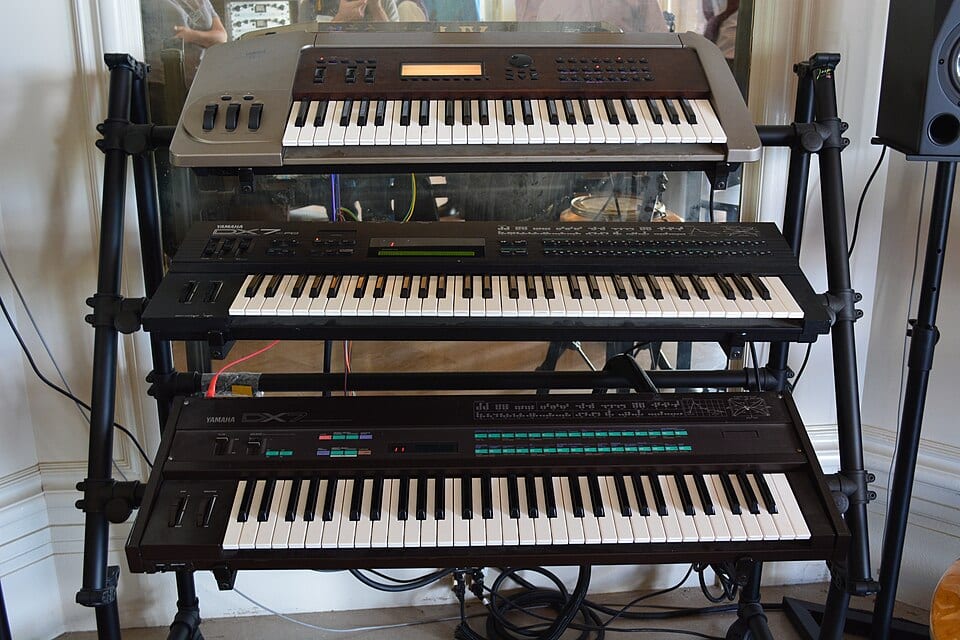
Sound On Sound’s July 1994 review listed “Polyphony: 2 notes maximum” and a UK price of £3,999, and noted that “‘Virtual Acoustics’ is Yamaha’s wording for what academics call Physical Modelling (PM)” (Sound On Sound, Yamaha VL1 review, July 1994). Yamaha’s own engineer later admitted “It didn’t do very well in terms of business at the time, but the physical modeling concept had far greater implications” (Yamaha, K’s Lab interview).

Korg’s Prophecy followed in 1995 with what Sound On Sound summed up as “physical modelling of plucked strings. And brass. And reeds” (Sound On Sound, Korg Prophecy review, October 1995). The Z1 of 1997 made the same engine polyphonic: “12-voice polyphonic, with each voice derived from a pair of physically modelled oscillators” (Sound On Sound, Korg Z1, August 1997).

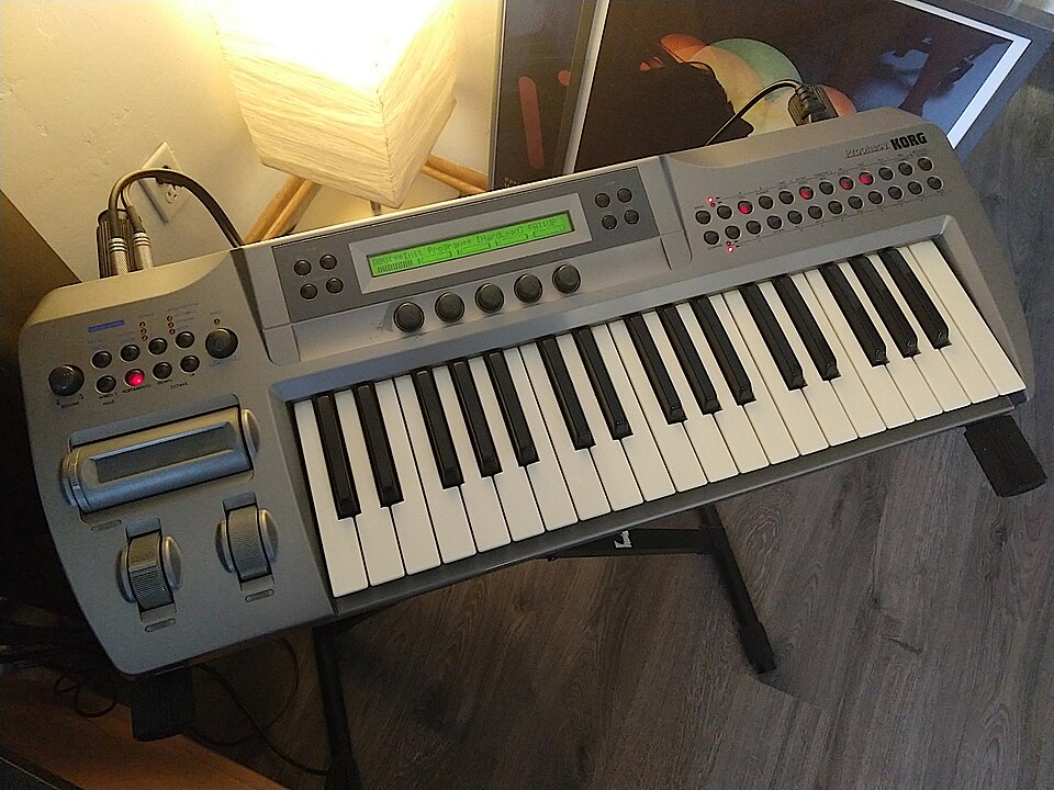
Hardware physical modeling then stayed a niche. Smith’s explanation: it “did not immediately meet with large commercial success, perhaps because wavetable synthesis required less computation”, and wavetable sounds were much easier to program. In the 1990s, “wavetable synthesis” mostly meant sample playback. The comeback came in software, once ordinary computers had CPU to spare; my analog vs digital synthesizers article covers that wider shift.

Where you find physical modeling today

Most people meet physical modeling as a plugin or a DAW instrument, not as hardware.

• Logic Pro Sculpture. Apple’s manual: “Sculpture is a synthesizer that generates sounds by simulating the physical properties of a vibrating string. This approach to tone generation is called component modeling” (Apple, Logic Pro User Guide). It arrived with Logic Pro 7, announced in September 2004 (Apple Newsroom, 2004).
• Ableton Tension, Collision and Electric. All three were made with Applied Acoustics Systems. Ableton’s manual says Tension “uses no sampling or wavetables”, and Collision models mallet percussion with beam, membrane, plate, pipe and tube resonators (Ableton, Live Instrument Reference). Tension and Electric came as add-ons with Live 7 in 2007 (Sound On Sound news, October 2007), Collision with Live 8 in 2009 (Ableton press release).
• Applied Acoustics Systems. AAS describes Chromaphone 3 as “a two-voice synthesizer based on physically modelled acoustic resonators” (AAS, Chromaphone 3); here voice means one of two layered sound engines, not two-note polyphony as on the VL1. AAS’s guitar instrument, Strum GS-2, offers “More than 100 acoustic guitar presets with a choice of nylon and steel strings and different body shapes”, plus electric guitars (AAS, Strum GS-2).
• Pianoteq and Objekt. Modartt released Pianoteq in August 2006 (Modartt news). Reason Studios launched Objekt in May 2023 and calls it “an open-ended physical modeling synthesizer” (Reason Studios, Objekt).
• Inside bigger synths. Arturia’s Pigments lists a Modal engine among “6 forms of synthesis: Modal, Granular, Wavetable, Sample, Harmonic and Virtual Analog” (Arturia, Pigments). AAS’s instruments, Pianoteq and Pigments are VST plugins for most DAWs; Sculpture and the Ableton instruments only run inside Logic and Live.

Hardware hasn’t disappeared. Arturia’s MicroFreak has a Karplus-Strong oscillator mode, and its manual explains that “Karplus-Strong is the name of the sound synthesis method developed by Kevin Karplus and Alex Strong at Stanford University” (Arturia, MicroFreak manual). In Eurorack, Mutable Instruments’ Rings and Elements are modal and string resonators. The company “has shut down in December 2022”, but its designs are published as “Open-source software and hardware” (Mutable Instruments). Expressive E’s Osmose runs Haken Audio’s EaganMatrix engine, which the maker says covers everything “from analog to physical modeling” (Expressive E, Osmose).

Which physical modeling synth is best depends on what you want to model. For mallets, bells and struck objects, look at resonator-based instruments such as Collision and Chromaphone, or a modal module such as Elements. For plucked and bowed strings, look at string models such as Tension, Strum or Sculpture (Chromaphone and Strum are the two I’ve used myself). For pianos and electric pianos, a dedicated model like Pianoteq. For wind instruments, the Yamaha VL line was the specialist: Yamaha says “The VL1 was created with reed instruments and other wind instruments in mind” (Yamaha, Innovation Road: VL1), and it came with a breath controller.

Not everything sold as modeling is physical modeling. “Roland first developed COSM for the VG-8 V-Guitar System, which was introduced way back in 1995” to model guitars, pickups and amps (BOSS Users Group). That’s circuit and amp modeling, closer to virtual analog than to a simulated string. Even Roland draws the line loosely: its V-Piano designer, Tadao Kikumoto, says the V-Piano’s approach “goes beyond the limits of physical modeling” (Roland Articles), so the label alone won’t tell you which kind of modeling you’re getting.

Strengths and limits of physical modeling

The big strength is expression. Smith writes that “Trained performing musicians generally prefer the expressive richness of a computational physical model”. Because the model is the whole instrument, Sound On Sound’s VL1 review noted, “it also produces realistic transitions between notes, not just the notes themselves.” Pianos gain too. Sound On Sound’s V-Piano review highlights “the absence of velocity switching inherent in the sampled alternative” (Sound On Sound, Roland V-Piano, May 2009). Sound On Sound’s first Pianoteq reviewer believed the sustain pedal’s effect is “impossible to replicate using a fixed menu of samples.”

The limits are just as real.

• CPU. Reviewing Pianoteq 3.5, Sound On Sound warned “you’ll need a dual- or multi-core processor for best performance: this modelling is a CPU-intensive business” (Sound On Sound, February 2010).
• Programming. Stanford’s own licensing office found that “physical modeling voice development was quite a difficult undertaking” (Stanford OTL, Sondius case study). Apple says Sculpture “requires a more measured approach to sound creation than a traditional synthesizer design.”
• Playing. Physical models want to be played like the instrument. Sound On Sound’s Prophecy review warned that “simply pressing down the notes will produce a sound rather like a synthesized saxophone, or a poorly programmed Moog.” Perfect Circuit notes that the approach “required an extended controller paradigm, one that went beyond the note-on/velocity and even aftertouch” (Perfect Circuit). Breath control, aftertouch and a well-used modulation matrix do a lot of the work.

How to start a physical modeling patch

Most physical modeling instruments use the same building blocks under different names. Think in terms of exciter, resonator and damping, and these starting points carry across plugins:

• Plucked string: a short, bright exciter (pick or noise burst), a string resonator, moderate damping. Map velocity to exciter brightness so soft notes come out darker.
• Struck bar or bell: a mallet exciter into a beam or plate resonator. Raise the inharmonicity or change the material for bell-like partials, and move the strike position to change which modes ring.
• Blown pipe: a noise exciter with a slow attack into a tube or pipe resonator. Put breath, aftertouch or the mod wheel on exciter level, since a wind sound lives on continuous control.
• Impossible instrument: keep the exciter and swap the resonator for something no factory could build, such as a plucked membrane or a bowed plate the size of a room. This is where physical modeling turns into sound design rather than imitation.

Shape the result with the instrument’s own envelopes or an ADSR on the exciter. If you also work with virtual analog, wavetable or granular synthesis, a physical model makes a good layer: the modeled pluck or strike gives the attack a life the other engines find hard to fake.

Frequently asked questions

What is physical modeling synthesis in simple terms?

Physical modeling synthesis makes sound by simulating an object that vibrates. An exciter such as a pluck, strike, bow or breath drives a resonator such as a string, tube or plate, and the synth computes the result as you play. It stores a model, not recordings; Pianoteq, for example, downloads at about 50 MB.

What is the Karplus-Strong algorithm?

Karplus-Strong is a plucked-string algorithm. A delay line of N samples is filled with noise and played in a loop, and every pass averages neighboring samples. The noise turns into a decaying tone at a pitch of the sample rate divided by N + 1/2. Karplus and Strong developed it around 1979 and published it in 1983.

Is physical modeling better than sampling?

Neither is better in general. Sampling captures specific notes of one real instrument and is light on the CPU, but it needs gigabytes and switches between fixed layers. Physical modeling needs only megabytes, reacts continuously to playing and allows impossible instruments, but it costs more CPU and is harder to program.

Is virtual analog a type of physical modeling?

Not in the usual sense. Virtual analog simulates oscillators, filters and circuits of analog synths, while physical modeling simulates acoustic objects like strings, tubes and plates. Some makers call circuit simulation modeling too, which blurs the line. Roland’s COSM, for example, first appeared in 1995 to model electric guitars, pickups and amplifiers rather than acoustic instruments.

Which synths use physical modeling?

Classic hardware includes the Yamaha VL1 from 1994 and the Korg Prophecy and Z1. Today most physical modeling runs in software: Logic Pro’s Sculpture, Ableton’s Tension, Collision and Electric, AAS Chromaphone and Strum, Pianoteq and Reason’s Objekt. In hardware, the Arturia MicroFreak and the Expressive E Osmose carry it on, alongside Mutable Instruments’ now-discontinued Rings and Elements.

Why is physical modeling so CPU-intensive?

A physical model computes the vibration of the instrument for every sample instead of reading back a recording. Simple string models are cheap, but detailed ones are not. A 3D room model from the NESS research project needed 240 processor cores for about 80 minutes to produce one second of audio, and a 2010 Pianoteq review recommended a multi-core CPU.

Back to Music Production Terms Index Page